Galaxy Zoo Challenge - Image Classification with PyTorch

This is an image classification project that I completed for my independent study at Old Dominion University. I’m interested in astronomy and chose to do Kaggle’s Galaxy Zoo Challenge.

I’m going to walk you through my workflow for this project, including exploratory data analysis, image processing, and finally building a convolutional neural network (CNN) with PyTorch.

View the source Jupyter Notebook (HTML), which contains the full source code as well as my learning notes. Please excuse the spelling, as Jupyter does not have spellcheck!

Index

1. Tools Used
2. Project Background
3. Exploratory Data Analysis
4. Benchmarking
5. Preprocessing
6. Convolutional Neural Network
7. Building the Model
8. Closing Thoughts

Tools Used

• Numpy
• OpenCV
• Pandas
• Python Image Library
• PyTorch
• Scipy
• Scikit-Learn

Project Background

This project is based on the Galaxy Zoo Challenge on Kaggle. Galaxy Zoo is a project to describe galaxies in the night sky using an innovative crowdsourcing tool, where users answer a series of questions about the images they are looking at. The dataset consists of 61,578 images with corresponding labels.

The labels represent 37 classes of the format “ClassA.B”, where A represents the questions being as (from 1 to 11) and B represents the choices at the given level. This is different than a typical classification problem because each class represents an attribute, and most images will contain multiple attributes. The values represent the confidence of the crowd that a given answer is correct, from zero to one. The decision tree does not show every question to the user, but rather the questions shown are based on the previous answers.

Figure 1 shows a graphical representation from the Galaxy Zoo 2 research paper.

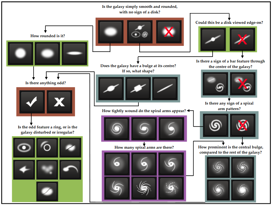
Figure 1: Willett, K. W., Lintott, C. J., Bamford, S. P., Masters, K. L., Simmons, B. D., Casteels, K. R. V., … Thomas, D. (2013). Galaxy Zoo 2: detailed morphological classifications for 304 122 galaxies from the Sloan Digital Sky Survey. Monthly Notices of the Royal Astronomical Society, 435(4), 2835–2860. doi: 10.1093/mnras/stt1458. Retrieved from [https://arxiv.org/abs/1308.3496](https://arxiv.org/abs/1308.3496)

My objective is the same as the Kaggle leaderboard scoring function, optimize the element-wise root mean-squared-error (RMSE). To evaluate that, I wrote the below function.

def RMSE(pred, truth):
    return np.sqrt( np.mean( np.square(
                np.array(pred).flatten() - np.array(truth).flatten() )))

Exploratory Data Analysis

The objective of my exploratory data analysis was to get a better understanding of the dataset to better inform my preprocessing and deep learning strategies. I wanted to learn a bit about how the classes are distributed as well as how the galaxies are displayed in the images.

The first thing I looked at was the instances of all classes where the confidence level was above 0.5. This is interesting to me because it will show me which classes are common and which are sparse, and the main actionable takeaway is whether I needed apply weights to the loss function. If the classes were all evenly distributed, I could use and out of the box loss function. If not, I would need to write one that applies weights to prevent the neural network from over-prioritizing classes where there isn’t enough data to effectively learn.

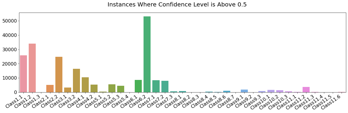
Figure 2: Class counts where confidence level is 0.5 or above.

As you can see, there are a few dominant classes, a number of somewhat sparse classes, and a few extremely sparse classes. I also dug into the nine terminal classes, answers where the decision tree terminates.

Class1.3: 44 Class6.2: 53115 Class8.1: 886 Class8.2: 4 Class8.3: 16 Class8.4: 301 Class8.5: 202 Class8.6: 1022 Class8.7: 27

There are three ways the decision tree terminates: not a galaxy, not an odd galaxy, and if odd, what type of oddity is present. As we can see, nearly every image does display a galaxy and an overwhelming majority, about 86%, are not odd. Of those that are odd, most fall into only two categories.

The sparse classes are non-viable, and to compensate for this I wrote the following PyTorch loss function:

weights = torch.tensor(np.sum(y_train, axis=0) / np.sum(y_train))

def weighted_mse_loss(output, targets, weights):
  # Arguments are all PyTorch tensors
  loss = (output - targets) ** 2
  loss = loss * weights.expand(loss.shape) # broadcast (37,) weight array to (n, 37).
  loss = loss.mean(0)
  return loss.sum()

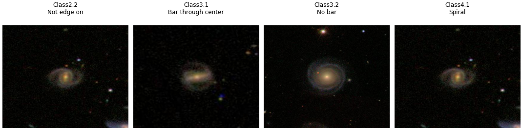
Next, I took a look at what these images actually look like. I selected the image with the highest confidence level for each class and drew them with Pyplot.

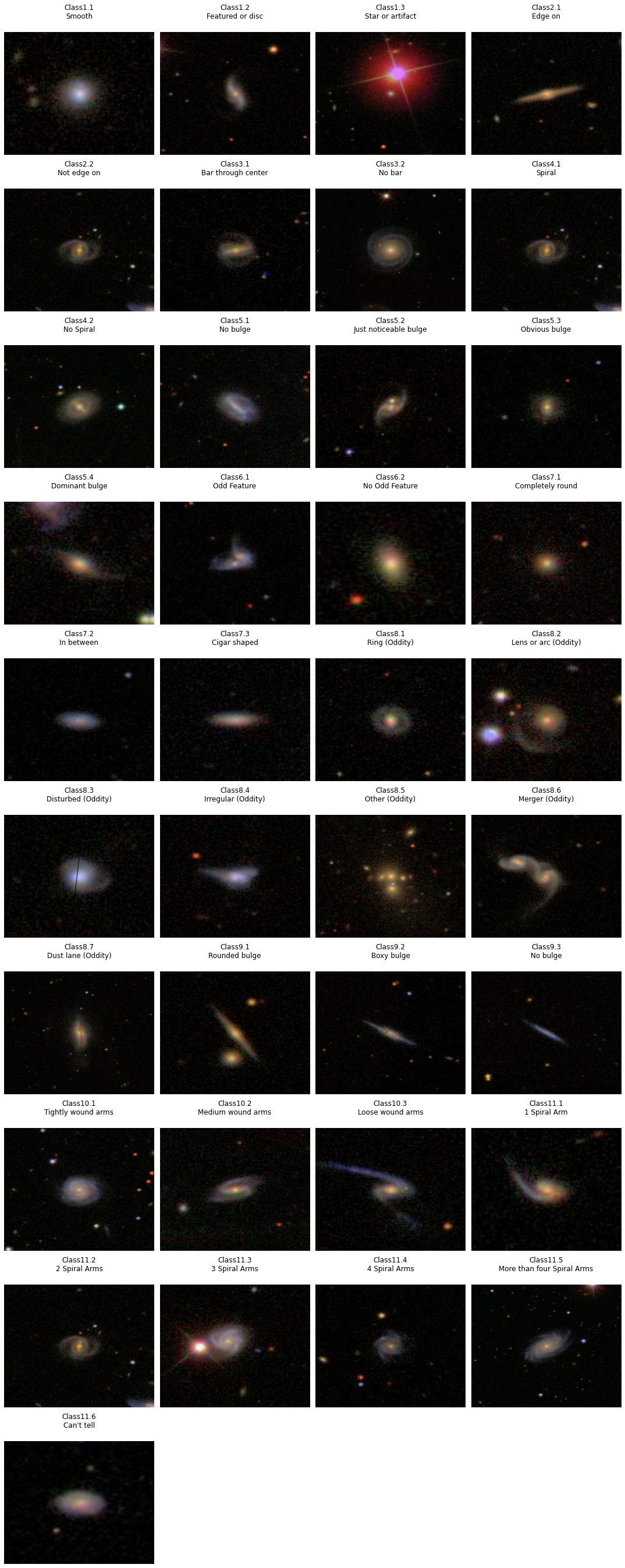
Figure 3: The image with the maximum confidence level for each class in the dataset.

Super cool! I never get bored of looking at pictures like this.

I have two main takeaways here: First, it appears as though the galaxies tend to be centered in the image. And second, like space itself, the majority of each image tends to be empty black space. To test this hypothesis, I took the average of all images.

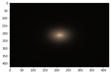
Figure 4: The average of all 61,578 images in the dataset.

The hypothesis appears correct. Because of this, I’m going to preprocess the images by extracting the region of interest to get the biggest bang for my buck in the convolution layers of my neural network.

I was also curious to see how strongly the crowd-sourced participants agreed with each other. Because we don’t have a single source of truth, we’re not really modeling which galaxies have which attributes but rather how confident the human scorers that a galaxy has a certain attribute.

To understand this better, I drew correlation matrices for the answers to each question as heatmaps.

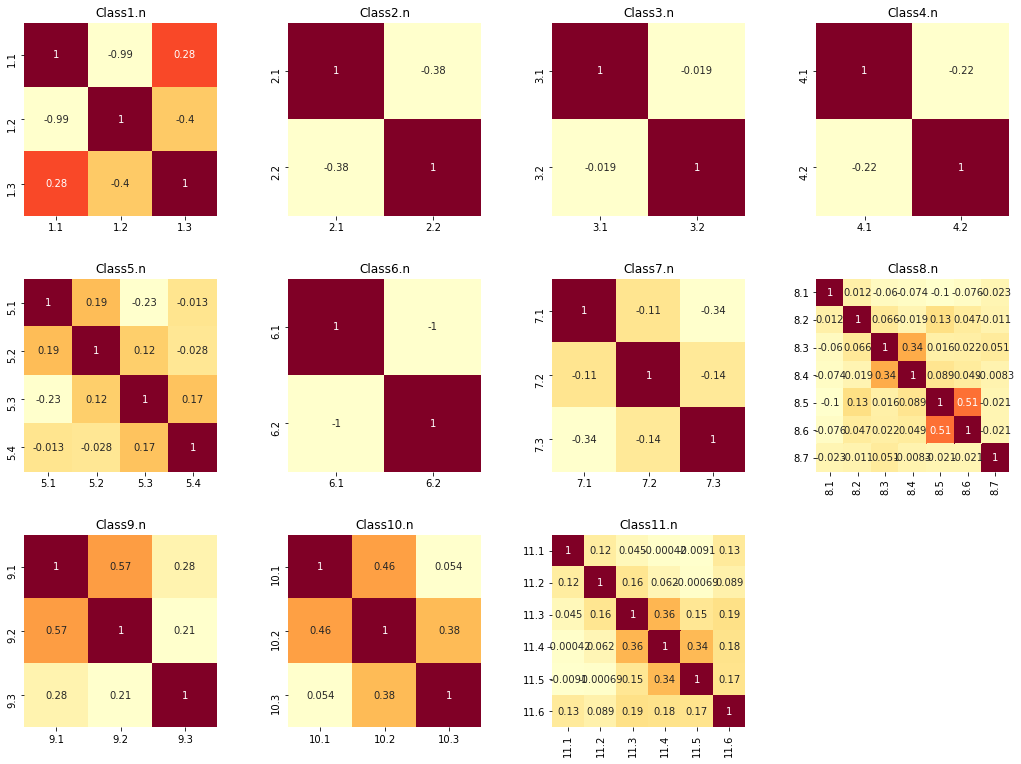
Figure 5: Correlation matrices for each of the eleven questions.

If the participants were mostly in agreement for a particular question, there will be very little correlation between the answers to each question. However if there is disagreement, then there will be a higher level of correlation.

This is important because because we’re modeling people’s decision-making process, and if they aren’t confident than it might be a challenge for our model to be confident.

Benchmarking

Though this is a heart a classification problem, the objective of modeling the confidence level of humans classifying the galaxies transforms it into a regression problem.

As mentioned above, I’m going to be using an element-wise root mean-squared-error (RMSE) scoring function. Unlike classification problems where things like confusion matrices, precision, recall, and F1 scores are easy to understand, RMSE is a bit more abstract. You can’t really say what a ‘good’ RMSE score is, rather you have to set a baseline benchmark for the minimum possible performance and improve from there.

On the Kaggle leaderboard there is a “central pixel benchmark” of 0.16194. This is found by predicting the classes simply based on the average scores for images with the same central pixel. It seems like a decent score fall somewhere between 0.10 and 0.12 with the winner achieving 0.07941. With my time constraint of just a week for the project I don’t think I’m going to hit the winning score, but I’d be happy falling comfortably within the top half of scores.

But since this is a learning exercise, I decided to make my own benchmark. I chose three strategies:

• Linear regression based on the central pixels
• Linear regression based on the average pixels
• A sanity check of just the average confidence to see if the previous two have any meaning

def average_color(pic):
    return np.sum(pic, axis=(1,2)) / (pic.shape[1] * pic.shape[2])

def center_pixel(pic):
    return pic[:,int(pic.shape[1] / 2),int(pic.shape[2] / 2),:]

lr = sklearn.linear_model.LinearRegression()
lr.fit(X_train, y_train)
pred = lr.predict(X_test)

The results?

• Central Pixel RMSE: 0.1564
• Average Pixel RMSE: 0.1599

Both are better than the provided benchmark! But does this mean anything?

• Just the Average Confidence RMSE: 0.1639

Linear regression only beat just using the class average for every image by about 4.6%. Looks like we’ll have to use deep learning after all!

Preprocessing

The problem with these images is that they have a lot of empty black space, and as I’m building a computationally intense neural network I really don’t want to have billions of operations analyzing nothing. My strategy was to find the region on interest from each image and crop it with a 20% pad on each side and then save as a 64x64 pixel PNG. I did this by analyzing all of the contours of luminescence in the image, bounding them with a rectangle, and then finding the biggest rectangle. The result was a much tighter crop, and as a happy side effect it introduced some variance to the position of the center pixel.

DATA = 'source files'
DIR_64 = 'output for 64x64 images'

padding_size = 0.2

for image in labels.GalaxyID:

    im = cv2.imread(DATA + image)
    im2 = cv2.cvtColor(im, cv2.COLOR_RGB2GRAY)
    ret, thresh = cv2.threshold(im2, 10, 255, 0)
    contours, hierarchy = cv2.findContours(thresh, cv2.RETR_LIST, cv2.CHAIN_APPROX_SIMPLE)

    ROI = (0,0,0,0) # Region of interest
    ROI_area = 0
    for contour in contours: # cv.RETR_LIST exports contours as a list.
        x, y, width, height = cv2.boundingRect(contour)
        area = width * height
        if area > ROI_area:
            ROI_area = area
            ROI = (x,y,width,height)

    x, y, width, height = ROI

    if width > height:
        pad = int(width * padding_size)
    else:
        pad = int(height * padding_size)

    if (y-pad >= 0 and
        x-pad >= 0 and
        y + max(width, height) + pad < im.shape[1] and
        x + max(width, height) + pad < im.shape[0]):
        crop = im[y-pad:y+max(width,height)+pad,x-pad:x+max(width,height)+pad]
    else:
        crop = im

    image = image.replace('jpg','png') # I don't want to multiply the compression loss. meme.jpg.jpg.jpg

    cv2.imwrite(
        DIR_64_WIDE + image,
        cv2.resize(crop, (64,64), interpolation=cv2.INTER_AREA)
    )

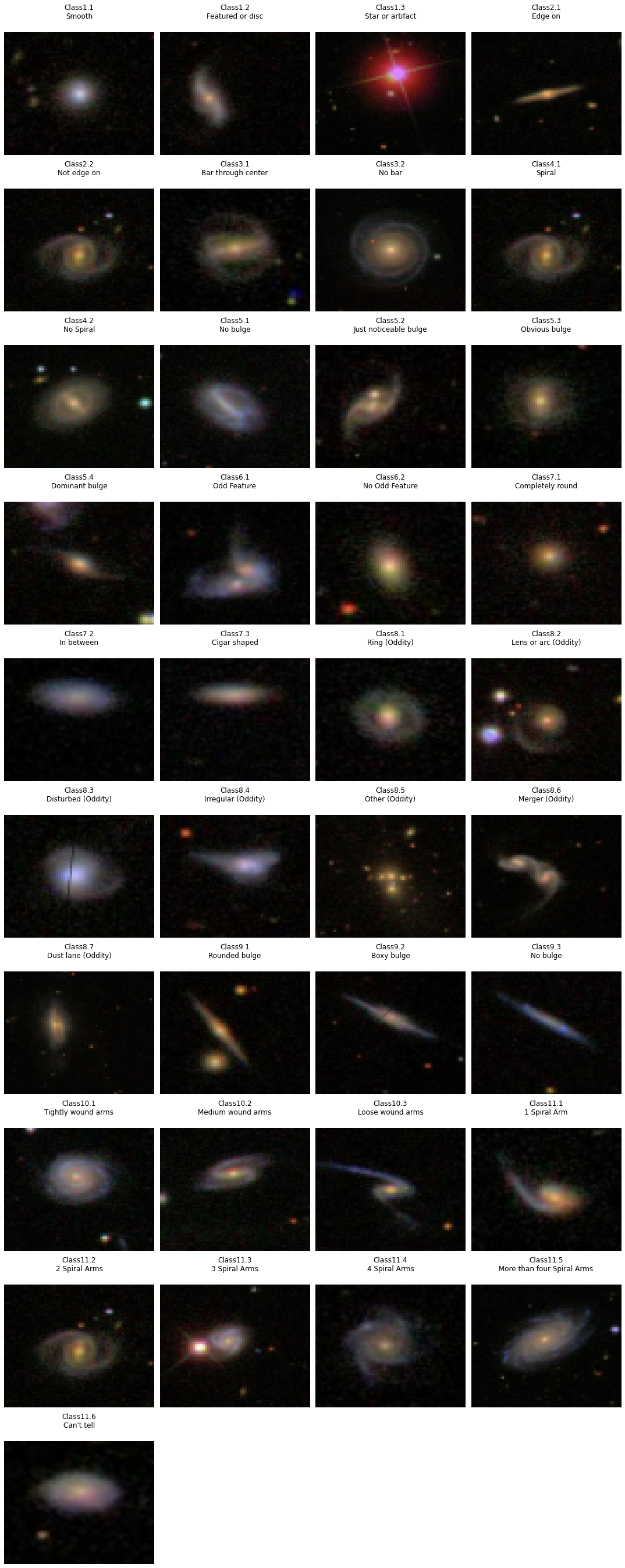
Figure 6: Images with the maximum confidence level from each class cropped around the region of interest.

Convolutional Neural Network

I’m going to use a convolutional neural network (CNN) for this problem. CNNs are uniquely suited for image classification problems because they can explore local relationships between pixels rather than looking at the whole picture all at once. I’ll explain more about that below.

In PyTorch, a neural network is defined as a class where each layer is a parameter initialized by a constructor with a forward propagation method. Input data is propagated forward through the network to make a prediction. Then it is evaluated by an error function, and the error is back-propagated through the network to update the weights.

Neurons

A neural network is composed of layers of neurons, which are a simple linear equation wrapped in an activation function. The output of each neuron is connected to one or more neurons in the subsequent layers depending on the architecture of the network.

$z = wx + b$   <- The linear equation

Where:

• $z$ = output
• $w$ = weight
• $x$ = input
• $b$ = bias

This information is stored in tensors (where the popular library TensorFlow got its name), which are often implemented as multidimensional arrays. In PyTorch, the tensor interface is modeled after the Numpy interface. A neuron has individual $w$ and $b$ values for each connection to another neuron in subsequent layers. A neural network is composed of many of these tensors connected in layers or as a graph. In the case of a convolution layer, there is a many to one relationship where outputs of neurons in a local area feed into a single neuron in the next layer. In a densely connected layer, or fully connected layer, each neuron is connected to every neuron in the subsequent layer.

That is the basic idea behind an Artificial Neural Network (ANN) or multilayer perceptron, and other architectures build off of this with different types of layers and structures between layers.

Activation Functions

Why can’t we just use the linear equation for neurons? The goal of a neural network is to create a non-linear decision boundary, it’s basically a non-linear function approximator. But there’s an interesting property of linear functions: the composition of two linear functions is always a linear function. If we were to use a linear activation function, no matter how many layers we create in the network the final result will always result in a linear function $w’x + b’$. We end up with a more computationally expensive linear regression model that consolidates a large number of features.

That’s neither interesting or useful when we’re classifying an image. We need something that explores complex relationships not only between the input features (pixels), but between the layers upon layers of these neurons. Remember that the task we’re trying to solve is approximating the process that happens in the human eye and brain between looking at a picture of a galaxy and clicking the answer to a question about that galaxy. To accomplish non-linearity, need to wrap our linear equation in an activation function that breaks linearity.

The most popular activation function for problems like this is a Rectified Linear Unit, or ReLU. This is extraordinarily simple:

$\sigma(x) = max(x,0)$

If the output is greater than zero, we simply use the output of the linear equation. If not, we use zero. Despite being simple, this is the most effective activation function for breaking linearity in a regression problem. It does have a few pitfalls, one being that a neuron can “die” or effectively be zero for any state. This can be solved with a Leaky ReLU, or replacing zero with a tiny multiple of x like this:

$\sigma(x) = max(x,0.005x)$

This isn’t a one-size-fits-all solution. For regression problems where our target is a probability, like this one, we can use a sigmoid function. This is guaranteed to output a number between 0 and 1.

$\sigma(x)= \frac{1}{1+e^{-z}}$

Convolution Layers

Convolution layers composed of kernels, or image filters. Filters pass over an image in steps, creating a new image where each pixel is the convolution of the filter matrix and a subsection of the image. Convolution is a matrix operation denoted by an asterisk $*$ that is in essence a weighted combination of two matrices. It passes in overlapping steps, and the output matrices lose a couple pixels based on the size of the kernel (one pixel on each edge for a 3x3 kernel) unless padding is applied.

These kernels allow the network to analyze local relationships between pixels rather than looking at the entire image.

One typical filter is a sharpening filter, in 3x3 form here, where n is the level of sharpening to be applied.

  0   -1   0

  -1   n   -1

  0   -1   0

Anyone familiar with image processing will recognize this kernel. But what makes a CNN powerful is that the convolution layers built from neurons will in effect learn new filters that are uniquely fitted to identifying and understanding features in the images. It will likely learn an edge detection filter and other standard filters, but it will also learn unique filters that pick up on subtle things.

The tensor in a convolution layer can contain multiple kernels. In effect, when we forward propagate through a convolution layer we’re creating one new matrix for each kernel.

Pooling

When we filter an input matrix through these feature maps, we retain the same dimensionality. But the real power of a convolutional neural network comes from extracting features from an original input image using feature maps, and then extracting subsequently more abstract features from combinations of the outputs.

After each convolution layer, we are increasing the width of our network, that is the number of filtered images. As we add on layers, we begin to suffer from the curse of dimensionality and the number of neurons explodes. It becomes extremely computationally expensive, and carrying that extra data hurts more than helps.

Because our objective with the learned kernels is to recognize patterns, reducing the size of the matrices effectively allows the neural network to zoom out and look at relationships between features recognized at previous convolution steps.

Remember that our ultimate goal is to understand the relationship between the pixels in an image and ultimately turn that information into 37 answers to 11 questions. Imagine looking very close at a picure of a car. Looking through a magnifying glass, you can recognize where edges and smooth surfaces are. Put down the magnifying glass and you can see where those edges make a car company logo, a unique headlight shape, a certain type of wheel. Step away from the photo and you can see the whole car made up of these components. You don’t need to see the pixels that define the boundary between the headlight and the hood to understand that the collection of parts you are looking at make either a Toyota or a BMW.

The theory behind a CNN is the same. As information flows through the network, higher level features are being extracted and it’s important to recognize a wider variety of features without getting bogged down in tiny details.

Pooling layers reduce the size our our matrices by breaking them down into grids, say 4x4, and reducing them each to a single pixes. There are many strategies, like max, sum, average, etc, and each have their strenghts and benefits.

Max performs kind of like a sharpening filter, and with our grayscale input images I think it will help our network pull out the most important features.

Fully Connected

Fully connected layers are flat layers with a full connection to every neuron in the previous and subsequent layers. Where the convolution layers explore local relationships, the fully connected layers begin to look at the whole picture. These layers are basically act as a non-linear function approximator.

The first fully connected layer takes the features detected by the convolution layers as input and the final fully connected layer outputs our prediction.

Regularization

The dense connections in this part of the network are great at analyzing the relationships between features in an image and whatever we are trying to predict, but they do come with a downside. Sometimes they just memorize data and perform amazing on the training data set, but not so well on testing data.

Similar to how the Boston Dynamics robots learn to be more stable on their feet from employees kicking them down, the neural network becomes stronger when we disrupt it by shutting off neurons at random. This causes other neurons which may otherwise not be used for a particular decision to pick up the slack and find alternate ways of making that decision. This is a very common regularization strategy in deep learning.

Another regularization strategy is batch normalization. This is one of those funny things that works even though people are totally sure why it works. This is a PHD level topic, but my basic understanding is that it prevents major shifts in input data from having an outsized effect on the weights and balances. The step of updating the network parameters is called back propagation, where the hill we’re descending is a gradient of the loss function with respect to the weights. Batch normalization smooths out this gradient and prevents dramatic changes. The slower and more stable learning process is able to find solutions faster because you don’t have to waste steps correcting overshoots and major shifts in the weights.

Building the Model

Batch Generator

I’m working with limited RAM here, so it is necessary for me batch the data. I wrote a custom batch generator to accomplish this. While I did the major preprocessing beforehand and saved the data to storage, I reserved the faster preprocessing step of randomly rotating images for the batch generator to save on storage space.

def torch_batches(pics, labels, path=DATA, batch_size=30, rotate=False, fmt='png'):
    '''
    Generate batches of PyTorch tensors from a list of image filenames.
    DATA is a global variable with the path to the image folder.  
    '''
    angles = np.array([0,90,180,270])
    labels = torch.tensor(labels, dtype=torch.float32)
    l = len(pics)
    batches = int(l/batch_size)
    leftover = l % batch_size
    for batch in range(batches):
        start = batch * batch_size
        this_batch = pics[start:start+batch_size]
        batch_labels = labels[start:start+batch_size,:]

        if rotate:
            yield torch.tensor([scipy.ndimage.rotate(
                                plt.imread(path + pic, format=fmt),
                                reshape=False,
                                angle=np.random.randint(0,360)
                                )
                            for pic in this_batch], dtype=torch.float32).permute(0, 3, 1, 2), batch_labels, this_batch
        else:
            yield torch.tensor([ plt.imread(path + pic, format=fmt) for pic in this_batch], dtype=torch.float32).permute(0, 3, 1, 2), batch_labels, this_batch

Defining the CNN

PyTorch is a low-level deep learning library (it does a lot of other things to, it’s basically a GPU accelerated Numpy with machine learning and statistics modules that replaces matrices with tensors), meaning that it does not automatically build the structure of your neural network like a higher-level library like Keras would. This is a challenge because you have to be accurate in calculating the shape of your data as it flows through the network.

The get_output_width() function and definition of the variables above the Net() class definition made this much easier and allowed me to make adjustments and experiment more easily.

The network consists of five layers:

• Convolution with 3 channels in and 64 filters. ReLU activation.
• Covolution with 96 filters and batch normalization. ReLU activation.
  • flatten non-index dimensions
• Fully connected layer with dropouts and 1/8 the number of output neurons as previous convolution layer. ReLU activation.
• Fully connected layer with dropouts and 1/4 the number of output neurons as previous layer. ReLU activation.
• Fully connected layer with 37 outputs, one for each class. Sigmoid activation.

def get_output_width(width, kernel, padding, stride):
    return int((width + 2 * padding - kernel - 1) / stride + 1)

classes = labels.columns[1:]

in_width = 64

kernel = 5
pool_kernel = 2
padding = int(kernel/2)
stride = 1

c1_in = 3
c1_kernel = 9
c1_out = 64
c1_conv_width = get_output_width(in_width, c1_kernel, int(c1_kernel/2), stride)
c1_pooled_width = get_output_width(c1_conv_width, int(pool_kernel/2), 0, pool_kernel)

c2_kernel = 5
c2_out = 96
c2_conv_width = get_output_width(c1_pooled_width, c2_kernel, int(c2_kernel/2), stride)
c2_pooled_width = get_output_width(c2_conv_width, pool_kernel, int(pool_kernel/2), pool_kernel)

full_1_in = c2_out * c2_pooled_width * c2_pooled_width
full_1_out = int(full_1_in / 8)
full_2_out = int(full_1_out/4)
full_3_out = len(classes)


class Net(nn.Module):
    def __init__(self):
        super(Net, self).__init__()
        '''
        These are the layers in the network, and their attributes are the
        weights and biases of the neurons.
        '''
        self.conv1 = nn.Conv2d(in_channels=c1_in,
                               out_channels=c1_out,
                               kernel_size=c1_kernel,
                               stride=stride,
                               padding=padding,
                               padding_mode='zeros')
        self.pool = nn.MaxPool2d(pool_kernel)
        self.conv2 = nn.Conv2d(in_channels=c1_out,
                               out_channels=c2_out,
                               kernel_size=c2_kernel,
                               stride=stride,
                               padding=padding,
                               padding_mode='zeros')
        self.conv2_bn = nn.BatchNorm2d(c2_out)
        self.fc1 = nn.Linear(full_1_in, full_1_out)
        self.fc2 = nn.Linear(full_1_out, full_2_out)
        self.fc3 = nn.Linear(full_2_out, full_3_out)
        self.dropout = nn.Dropout(p=0.15)

    def forward(self, x):
        x = self.pool(F.relu(self.conv1(x)))
        x = self.pool(F.relu(self.conv2_bn(self.conv2(x))))
        x = x.view(x.size()[0],-1)
        x = F.relu(self.dropout(self.fc1(x)))
        x = F.relu(self.dropout(self.fc2(x)))
        x = self.fc3(x)
        return x

net = Net()

Training the CNN

I trained the CNN with the Adam optimizer. It’s a little faster than stochastic gradient descent with comparable performance. I’m loading images from storage into memory in large batches because that’s more efficient, but I’m training in smaller mini batches to prevent dramatic gradient updates. The batch size is actually a regularization strategy for neural networks.

I trained the model over five epochs using the ROI cropped photos with random rotation.

optimizer = optim.Adam(net.parameters())
loss_history = []
batch_size = 1024
mini_batch_size = 64

for epoch in range(1,6):
    batch_no = 1

    datagen = torch_batches(X_train,
                        y_train,
                        path=DIR_64_WIDE,
                        batch_size=batch_size,
                        rotate=True)

    for images, targets, _ in datagen: # big read from storage
        for mini_batch in range(int(batch_size/mini_batch_size)):
            start = mini_batch*mini_batch_size
            if start >= images.shape[0]:
                break
            finish = start + mini_batch_size
            optimizer.zero_grad()   
            outputs = net(images[start:finish])
            loss = weighted_mse_loss(outputs, targets[start:finish], loss_weight)
            loss.backward()
            optimizer.step()
        batch_no += 1
        loss_history.append((epoch, batch_no, loss.item()))

The result? A respectably decent score of 0.11025! I would have placed 78th in the competition.

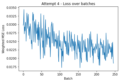
Figure 7: Weighted MSE loss over batches of 1024 images.

Closing Thoughts

I had fun working on this project. The bulk of the work was done within a week, and it was my first time using OpenCV and PyTorch. They’re both great libraries that are very approachable and easy to learn, as the Python data science community writes great documentation.

Given more time I would experiment more with both the preprocessing, particularly with more variance with the central pixel and maybe having the region of interest partially obscured around the edge to make the model more robust, as well as with the architecture of the neural network. I may revisit the project later on.

All in all, a great way to kick of my final semester’s independent study!