
Toxic Comment Classification - Natural Language Processing
The Jypyter notebooks and a report in PDF format can be found on my GitHub page here.
I. Definition
Project Overview
Platforms that aggregate user content are the foundation of knowledge sharing on the Internet. Blogs, forums, discussion boards, and, of course, Wikipedia. But the catch is that not all people on the Internet are interested in participating nicely, and some see it as an avenue to vent their rage, insecurity, and prejudices.
Wikipedia runs on user generated content, and is dependent on user discussion to curate and approve content. The problem with this is that people will frequently write things they shouldn’t, and to maintain a positive community this toxic content and the users posting it need to be removed quickly. But they don’t have the resources to hire full-time moderators to review every comment.
This problem led the Conversation AI team1, owned by Alphabet, to develop a large open dataset of labeled Wikipedia Talk Page comments, which will be the dataset used for the project. The dataset is available through Kaggle2.
The dataset has six labels that represent subcategories of toxicity, but the project is going to focus on a seventh label that represents the general toxicity of the comments.
The project will be done with Python and Jupyter notebooks, which will be attached.
Disclaimer: The dataset has extremely offensive language that will show up during exploratory data analysis.
Problem Statement
The goal is to create a classifier model that can predict if input text is inappropriate (toxic). 1. Explore the dataset to get a better picture of how the labels are distributed, how they correlate with each other, and what defines toxic or clean comments. 2. Create a baseline score with a simple logistic regression classifier. 3. Explore the effectiveness of multiple machine learning approaches and select the best for this problem. 4. Select the best model and tune the parameters to maximize performance. 5. Build a the final model with the best performing algorithm and parameters and test it on a holdout subset of the data.
Metrics
Unfortunately for the problem, but fortunately for the Wikipedia community, toxic comments are rare. Just over 10% of this dataset is labeled as toxic, but some of the subcategories are extremely rare making up less than 1% of the data.
Because of this imbalance, accuracy is a practically useless metric for evaluating classifiers for this problem.
The Kaggle challenge based on this dataset uses ROC/AUC, or the area under a receiver operating characteristic curve, to evaluate submissions. This is a very generous metric for the challenge, as axes for the curve represent recall (a.k.a. sensitivity), the ratio of positive predictions to all samples with that label, and specificity, the ratio of negative predictions to all negative samples. This metric would work well if the positive and negative labels were relatively even, but in our case, where one label represents less than a third of a percent of the data, it’s too easy to get a high score even with hardly any true-positive predictions.
Instead, I propose using an F1 Score, which severely penalizes models that just predict everything as either positive or negative with an imbalanced dataset.
Recall, as mentioned earlier, is the ratio of true positive predictions to positive samples. Precision, on the other hand, is the ratio of true positive predictions to the sum of all positive predictions, true and false.
Each gives valuable insight into a model’s performance, but they fail to show the whole picture and have weaknesses where bad models get high scores. Predicting all positive values will bring recall up to 100%, while missing true positives will be penalized. Precision will harshly penalize false positives, but a model that predicts mostly negative can achieve a high precision score whether or not the predictions are accurate.
The F1 score is a harmonic average between precision and recall. This combines the strengths of precision and recall while balancing out their weaknesses, creating a score that can fairly evaluate models regardless of dataset imbalance.
My justification for focusing on any_label as the target is that distinctions between the specific labels are relatively ambiguous, and that there is greater value focusing on general toxicity of a comment to more reliably flag it for review. This will reduce the workload of moderators who will ultimately be making the final call, and the specific category more relates to the consequences for the commenter rather than whether or not the comment should be deleted.
II. Analysis
Data Exploration This dataset contains 159,571 comments from Wikipedia. The data consists of one input feature, the string data for the comments, and six labels for different categories of toxic comments: toxic, severe_toxic, obscene, threat, insult, and identity_hate. The figure on the following page contains a breakdown of how the labels are distributed throughout the dataset, including overlapping data. As you can see in the breakdown, while most comments with other labels are also toxic, not all of them are. Only “severe_toxic” is clearly a subcategory of “toxic.” And it’s not close enough to be a labeling error. This suggests that “toxic” is not a catch-all label, but rather a subcategory in itself with a large amount of overlap. Because of this, I’m going to create a seventh label called “any_label” to represent overall toxicity of a comment. From here on in, I’m going to refer to any labeled comments as toxic, and the specific “toxic” label (along with other labels) in quotation marks.
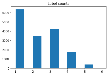
Fig 1: Label Counts
Only 39% of the toxic comments have only one label, and the majority have some sort of overlap. I believe that because of this, it will be much more difficult to train a classifier on specific labels than whether or not they are toxic. This ambiguity and the lack of explanation around it is what led me to select an aggregate label of general toxicity, what I’ve called “any_label,” as the target. 16225 out of 159571 comments, or 10.17%, are classified as some category of toxic.
1595 severe_toxic comments. (1.00% of all data.)
- 1595 or 100.00% were also toxic.
- 1517 or 95.11% were also obscene.
- 112 or 7.02% were also threat.
- 1371 or 85.96% were also insult.
- 313 or 19.62% were also identity_hate.
1405 identity_hate comments. (0.88% of all data.)
- 1302 or 92.67% were also toxic.
- 313 or 22.28% were also severe_toxic.
- 1032 or 73.45% were also obscene.
- 98 or 6.98% were also threat.
- 1160 or 82.56% were also insult.
15294 toxic comments. (9.58% of all data.)
- 1595 or 10.43% were also severe_toxic.
- 7926 or 51.82% were also obscene.
- 449 or 2.94% were also threat.
- 7344 or 48.02% were also insult.
- 1302 or 8.51% were also identity_hate.
7877 insult comments. (4.94% of all data.)
- 7344 or 93.23% were also toxic.
- 1371 or 17.41% were also severe_toxic.
- 6155 or 78.14% were also obscene.
- 307 or 3.90% were also threat.
- 1160 or 14.73% were also identity_hate.
478 threat comments. (0.30% of all data.)
- 449 or 93.93% were also toxic.
- 112 or 23.43% were also severe_toxic.
- 301 or 62.97% were also obscene.
- 307 or 64.23% were also insult.
- 98 or 20.50% were also identity_hate.
8449 obscene comments. (5.29% of all data.)
- 7926 or 93.81% were also toxic.
- 1517 or 17.95% were also severe_toxic.
- 301 or 3.56% were also threat.
- 6155 or 72.85% were also insult.
- 1032 or 12.21% were also identity_hate.
The correlation matrix below provides more insight into these overlapping categories. Threats are not likely to be severely toxic, nor are they likely to be racist or homophobic. But insults are often obscene, and identity hate really doesn’t have much overlap at all.
I believe the categories with significant overlap will be more difficult to predict, as they’ll have similar contributing features, but “identity_hate” will have more unique attributes and be easier to predict.

Fig 2: Correlation Matrix Heatmap of Labels
So what do these comments look like? Let’s look at a few.
Clean comments:
- “By baysian logic the picture is quite relavent. Only someone so opposed to the Vietnam war, as to visit NVN, would support something as tawdry as WSI. The photo is contemporary to the time period of the WSI, and is a very defining picture of one of the key participants during the time period that WSI took place.”
- “Oppose. Other towers have articles, so this one should. 89.242.19.188”
- “This sounds like your opinion. I’m giving you National Geographic, and GW supporters give me the IPCC, a group of politicians who pick and choose articles that support the idea of anthropogenic global warming and discredit any scientist who dissents. The reason I toss the term ‘nazi’ around is that it seems this article is loosely guarded by (what I call) a ““gestapo”” that sits around with an arsenal of ““talk-back”” to shoot down anyone who dissents from the idea of man-made GW. I was talking about the Sun and how other planets are warming. In my book, this falls under the area of astronomy, which last I checked is a science. You seem to think science is only opinions that agree that man is causing global warming, and I’m sorry, I don’t agree with that.12.26.68.146”
So clean comments can be argumentative and can include name calling, but are generally positive discussions.
The IP addresses in comments are concerning, as that’s a data leak and could cause issues since we want the classifier to predict toxicity based on the content of the comments. Because of this, I’ve used a regular expression to strip all of the IP addresses from the dataset.
I’ve found one other data leak as well: usernames. Removing them without a database of users is an incredibly difficult task. But while removing them completely isn’t an option, the term frequency – inverse document frequency vectorizing strategy should minimize or even eliminate their influence on the model.
Toxic Comments:
- “your a cocksucker u can’t do anything to me”
- “What 3 minutes every now and then - I’m not compiling lists and spending fucking hours doing fuck-all because no one loves me - how many edits have you done? Let’s remember - you’re so stupid and indeed pathetic you don’t even use your own name”
- “again again again
- this is not going to stop……hmmmm a personal attack let me think……you are a big poo poo face and smell like a frog”
Various types of toxic comments seem to almost always be argumentative, though they don’t necessarily involve profanity. Traditional filters involve a database of profanity to screen comments, but this breaks down when legitimate comments discuss profanity and toxic comments have clean language.
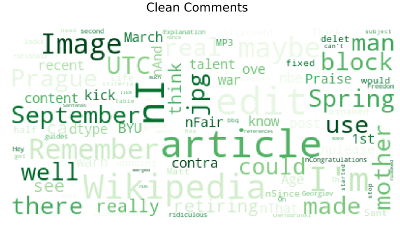
So what does a clean Wikipedia comment look like? I used a tokenizer with the standard stopwords to get the overall count of individual words and plotted the top 45.

Fig 3: Non-Toxic Comment Word Frequency
Article, page, please, think, edit, etc. The highest frequency words are about what you would expect from people discussing Wikipedia page edits and policy.
Now let’s look at what a bad comment looks like. Can you find the top two words from the clean comments? “Wikipedia” surprisingly comes in second, and “article” falls back quite a few spaces. The difference in the highest frequency vocabulary is stark.
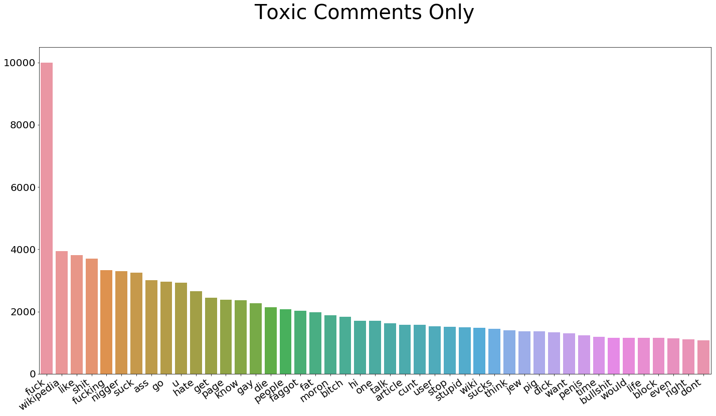
Fig 4: Toxic Comment Word Frequency
In addition to the words themselves, I’ve extracted some other attributes of the comments that show contrast between toxic and clean comments.
- Capitalization
Toxic comments are more likely to be either in all caps or have no capitalization at all. In an average clean comment, 5% of the characters are capital letters. In toxic comments, that number jumps to 14%. I think this feature will be extremely useful, especially with tree-based models due to it’s nonlinear nature. While the mean percentage of capital letters in toxic comments is almost triple that of clean comments, the medians are the same at 4%. This suggests that while clean comments are consistently capitalized, toxic comments have quite a few outliers. This is confirmed when browsing through the comments, as toxic comments are often all caps or not capitalized at all. - Comment Length
On average, clean comments are about a third longer than toxic comments. The average character count for clean comments is 404, while toxic comments average 303 characters. Looking at random samples, many clean comments have very long, well though-out answers. The median comment lengths are 128 characters for toxic comments and 216 characters for clean comments, suggesting that these longer comments make up a significant portion of the dataset for both types of comments. - Word Length
This one is a little closer, but there is a difference. Toxic comments average 4.1 characters per word, where clean comments average 4.4. But on a comment-by-comment basis this could be meaningful, as a visual scan shows that many of the toxic comments are more likely to use informal abbreviations like “u.” - Question Marks
My thought here is that more legitimate posts might have more question marks. But that assumption was wrong, as toxic comments have 50% more question marks per comment than clean comments. 0.6 versus 0.4. - Exclamation Marks
I made the opposite assumption about exclamation marks, and that paid off! Toxic comments have an average of 3.5 exclamation marks, while clean comments only have 0.3. This could be a very useful feature.
Algorithms and Techniques
As a natural language processing problem, is a classification task that involves high dimensionality data. I will vectorize the data and test multiple classification algorithms.
I will vectorize the text data using the term frequency – inverse document frequency (tf-idf) statistic. This technique takes into account not only the frequency of words or character n-grams in the text, it also takes into account the relevancy of those tokens across the dataset as a whole. The inverse document frequency reduces the weight of common tokens while boosting the weight of more unique tokens. I will establish a benchmark for performance with the top 10,000 words, and the number of tokens and the mix of words and character n-grams will be a parameter to tune for higher performance later on.
I will also create a number of engineered features containing various attributes of the comment text, such as average word length, capitalization, and number of exclamation points. I will run the benchmark test without these features and experiment with them to optimize the solution.
With the benchmark vectorization and features, I will experiment with multiple algorithms with default parameters to determine the most effective approach to the problem. The models I will use are:
- Logistic Regresssion (Benchmark)
- Multinomial Naive Bayes
- Support Vector Machine
- Support Vector Machine with Naive Bayes Features
- Light GBM
Recurrent neural networks work well on this problem and top Kaggle leaderboards, but I think deep learning approaches might be too resource intensive for an algorithm that has to run instantly every single time a comment is posted on one of the most popular websites on the Internet. A major requirement if this were a real-life business problem is efficiency. Additionally, adapting the model to secondary features would require stacking, which is a messy solution that increases the complexity of both training and predicting. I’ve used model stacking in Kaggle competitions before, and it comes at the expense of efficiency.
One more consideration is transparency, and this is the biggest aspect of the decision not to use neural networks for this application. I want to have the ability to easily audit the model to ensure that it isn’t picking up bias around race, gender, sexual orientation, culture, or unforeseen categories from the curators of the data. SVM, Naive Bayes, and LightGBM will make it much easier for a third party to analyze the impact of specific features on the model and make appropriate adjustments to combat bias.
I predict that there will be a toss-up between Logistic Regression and Support Vector Machines. Naive Bayes may have strong performance due to the dramatic difference between the the frequency distributions of the vocabulary between comments.
Support vector machine models are unique in that they find the boundaries between classes by looking at the distances between the separating line and the nearest point for each class, and are not effected by outliers. In this project I will be using the linear kernel. The kernel trick with support vector machines involves projecting data with complex or nonlinear boundaries into a higher dimension where they are linearly separable and drawing a hyperplane between them using a linear model algorithm. Imagine a 2D problem where you have a circular boundary between two classes and need to draw your decision boundary with linear regression. With the kernel trick you’d be projecting that flat dataset into the dimensions and ideally the circle would look more like a hill, allowing you to cut through it with a 2D plane and establish a linear boundary. The linear kernel is the most efficient of the kernels and is very resistant to overfitting, which I think may be an issue with the dataset.
LightGBM is a tree-based ensemble model that is trained with gradient boosting. The unique attribute versus other boosted tree algorithms is that it grows leaf-wise rather than level-wise, meaning that it prioritizes width over depth. Boosted tree can be confused with forest models, but there is an important distinction. Where forest models like Scikit-Learn’s RandomForest use an ensemble of fully developed decision trees, boosted tree algorithms use an ensemble of weak learners that may be trained faster and can possibly generalize better on a dataset like this one where there are a very large number of features but only a select few might have an influence on any given comment.
LightGBM is not a high performer on Natural Language Processing tasks, but I think it’s worth trying a tree-based model here due to the very large disparity between toxic and clean comments with the engineered features and top 30 words. There may be some great, reliable splits here. The reason it doesn’t perform well on NLP tasks is that it requires dense input data, and the nature of vectorizing text creates absolutely massive matrices filled mostly with zeros. It also has a relatively small number of features that it can focus on, while the vectorized text may contain over 20,000 features.
Support Vector Machine with Naive Bayes Features or Multinomial Naive Bayes may perform even better. The paper Baselines and Bigrams: Simple, Good Sentiment and Topic Classification3 experiments with this algorithm on a variety of types of datasets and found that Support Vector Machines performed exceptionally well at sentiment analysis on datasets with lengthy texts, such as full-length movie reviews. The same paper suggest that Multinomial Naive Bayes works better on snippets of text. Assuming an average sentence length of 75 to 100 characters, the Wikipedia dataset used in this project averages 2-4 sentences, which is more than a snippet but not exactly lengthy. Naive Bayes with SVM features was found to interpolate between Naive Bayes and Support Vector Machines, combining strengths of each.
After establishing a baseline score for each model, I’ll choose the best one or two, depending on how close they are, and tune the vectorization and model parameters to optimize performance.
Baseline
The baseline model is a Logistic Regression model fit to tf-idf vectorized comment text with using only words for tokens, limited to 10,000 features. The target value is any_label, but I also want to track the model’s performance on specific categories. But I do think that it’s important to note that my personal difficulty in perceiving the difference in specific categories when looking through comments is reflected in the model’s ability to specifically predict severe_toxic, threat, and identity_hate labels.
The cross-validated F1 scores for each label break down as follows:
- toxic score: 0.7192
- severe_toxic score: 0.3224
- obscene score: 0.7452
- threat score: 0.2069
- insult score: 0.6277
- identity_hate score: 0.2772
- any_label score: 0.7299
I also tested a baseline with the engineered features included.
- toxic score: 0.7235
- severe_toxic score: 0.3475
- obscene score: 0.7440
- threat score: 0.2029
- insult score: 0.6274
- identity_hate score: 0.2768
- any_label score: 0.7328
The scores are nearly identical, but this may not necessarily be the case for all models.
III. Methodology
Reproducibility
I am setting a few parameters at the top of my Jupyter notebook to ensure reproducibility of results, and these will be used in every appropriate instance. This will ensure that the output is exactly the same every time the notebook is run.
- seed (for random states) = 42
- k (for n_folds) = 5
Experiments that take a significant amount of time, such as Data Preprocessing
Cleaning
The dataset is relatively clean. There is a minor data leak, IP addresses appended to some comments. For various reasons, mainly that this data may slightly compromise the model’s ability to generalize to new data, I’ve used a regular expression to strip all IP addresses from comments.
Feature Engineering
During the exploratory data analysis, I found that many attributes of comments outside of the words themselves may be useful in predicting whether they are toxic. The features I added to the dataset are:
- Comment length in characters
- Percent of letters in a comment that are capitalized
- Average length of words in a comment
- Number of exclamation marks in a comment
- Number of question marks in a comment
Vectorization
As discussed previously, I am using a term frequency – inverse document frequency (tf-idf) statistic to vectorize text. The number of features and presence of character n-grams is a parameter to tune for model optimization.
Feature Scaling
The engineered features are normalized from 0.0 to 1.0. The tf-idf features are not scaled.
Implementation
Finding the Best Algorithm To compare the relative performances of each algorithm, I’m going to test them on the same preprocessed data as the benchmark, a tf-idf vectorized data with 10,000 features. The target is any_label, and the scores are F1 scores with five-fold cross validation.
- Logistic Regression: 0.7299
- With engineered features: 0.7328
- Engineered feature boost: 0.39%
- Multinomial Naive Bayes (NB): 0.6670 (0 predictions for threat category)
- With engineered features: 0.6734 (0 predictions for threat category)
- Engineered feature boost: 0.96%
- Support Vector Machine (SVM): 0.7703
- With engineered features: 0.7739
- Engineered feature boost: 0.47% boost
- Support Vector Machine with Naive Bayes Features (NB-SVM): 0.7804
- With engineered features: 0.7842
- Engineered feature boost: 0.49%
- LightGBM*: 0.7470
- With engineered features: 0.7573
- Engineered feature boost: 1.38%
* The other algorithms used default parameters, but LightGBM parameters were modified to better suit an NLP problem as the default parameters aren’t really suited to the problem like they are with other algorithms.
LightGBM Baseline Parameter Modifications:
- ‘num_leaves’: 64,
- ‘n_estimators’: 500,
- ‘max_depth’: 16
Not surprisingly, the engineered features gave the tree based model a larger performance boost than other models. The performance gain for other algorithms is modest, but it does come at an extremely minimal cost in terms of processing resources and training time so I would consider them worthwhile.
In terms of overall performance, NB-SVM is the strongest performer and SVM comes in at a close second. The naive bayes features gave SVM a 1.31% performance boost at a cost of about five times the training time. Around thirty-five seconds versus a little over three minutes, but the difference is minimal at prediction time and the gain is significant.
LightGBM also showed strong results with some tuning, but there is an issue with the model that prevents it from being a practical solution unless it’s performance is significantly higher than other models. Like all tree-based models, dense data is a firm requirement. Refining the text vectorization strategy is an important aspect of optimizing a natural language processing solution. Linear regression and support vector machines can run on sparse matrices which reduces their memory footprint, but LightGBM will see memory grow too fast converting sparse matrices into dense ones.
Refinement of the NB-SVM Model
Step 1: Optimize tf-idf vectorizer
Experiment with word and character level ngrams and maximum feature counts. All other parameters are fixed, and refinement steps will all use five-fold cross validation.
| Word Ngram | Word Max Features | Char Ngram | Char Max Features | Score |
| 1 | 10,000 | 0 | 0 | 0.7842 |
| 1 | 30,000 | 0 | 0 | 0.7926 |
| 1-2 | 30,000 | 0 | 0 | 0.7877 |
| 2-6 | 30,000 | 0 | 0 | 0.4042 |
| 0 | 0 | 3-7 | 20,000 | 0.7742 |
| 1 | 5,000 | 3-7 | 5,000 | 0.7962 |
| 1-2 | 15,000 | 3-7 | 5,000 | 0.7985 |
| 1-2 | 20,000 | 3-7 | 10,000 | 0.8005 |
| 1-2 | 20,000 | 3-5 | 10,000 | 0.8015 |
| 1-3 | 20,000 | 3-5 | 10,000 | 0.8013 |
The ideal seems to be a 20,000 word ngrams in range 1-3 and 10,000 char ngrams in range 3-5, in a tie with the same settings but a 1-2 word ngram. An added benefit of these parameters is that this is a relatively fast vector to calculate.
Step 2: Tune NB feature weight
The NB feature transformer class has a parameter ‘epsilon’ that controls the influence of the feature level probabilities on the input features. The default parameter is 1.0.
| NB Weight | F1 Score |
| 0.1 | 0.7966 |
| 0.2 | 0.7989 |
| 0.3 | 0.8003 |
| 0.4 | 0.8001 |
| 0.5 | 0.8008 |
| 0.6 | 0.8013 |
| 0.7 | 0.8007 |
| 0.8 | 0.8020 |
| 0.9 | 0.8019 |
| 1.0 | 0.8015 |
The weight of the features transformed by Naive Bayes doesn’t have much effect of the model’s performance, only about a 0.006% gain between 0.1 and 1.0. But at 1.0, it offers a nice 1.31% versus without it. My takeaway is that the information that this transformation introduces isn’t impacted much by the weight given to it, at least when combined with the SVM algorithm.
Step 3: SVM Parameter Tuning
Parameter 1: Kernel
SVMs have a number of parameter options. The root option is the kernel, and other options stem from there. So far, we’ve been using a linear kernel. A linear kernel fits best to datasets where the the dataset is linearly separable, and because this model vastly outperformed a well-tuned boosted tree model (LightGBM) I assume that it has a reasonable level of linear separation.
This is a large dataset, and a major benefit of the linear kernel is that is is a parametric model, meaning that it has finite dimensionality regardless of the size of the input data. The gaussian kernel is better suited for nonlinear datasets, but it comes at the cost of being a non-parametric model. As the input data grows, it becomes more expensive computational to for both training and prediction.
Result of testing gaussian kernel: 30+ minute training on a computer with 8 virtual processors and 52GB of RAM and a slow prediction step. This is not a viable solution and will not be further pursued.
Parameter 2: Penalty for error term
Going with the linear kernel, there is only one major parameter to tune: C. This is the coefficient for the L2 penalization. The default is 1.0, and I will test 0.5, 0.7, and 0.9.
| C | F1 Score |
| 0.3 | 0.8049 |
| 0.5 | 0.8054 |
| 0.8 | 0.8032 |
| 1.0 | 0.8015 |
Setting C to 0.5 instead of the default 1.0 gives a 0.51% performance increase.
IV. Results
Model Evaluation and Validation
The model has been trained, tested, and optimized using training and test subsets of the data. I will use an unseen holdout subset of the data to evaluate the model.
The F1 Score on the holdout data is 0.8072.
Because it’s performance is similar to the results obtained in the previous stage, I can confidently say that the model will generalize well to unseen data. Because it is a real world dataset with a huge variety of comments discussing a diverse range of topics and covering situations from informative posts to flame wars, this is probably one of the better scenarios for training a model on text.
The text vectorization strategy using Scikit-Learn’s TfidfVectorizer() class makes the model immune to unseen features, as they will be ignored.
Justification
The final model offers a significant performance boost over the benchmark linear regression model, about 11%. So far we’ve been talking in the abstract about F1 Scores, but now let’s dig into the real world performance and what those numbers actually mean.
This model has 96% accuracy. Now on the surface, that sounds great. But since this is a highly imbalanced dataset, that doesn’t mean a lot. In fact, if I had just created a model that predicted “0” for every single item, it would get an accuracy of 90%.
The real metric of how well the model performed at predicting a toxic comment is recall. This model achieved a recall score of 0.74, which means that it correctly 74% of the actual toxic comments as toxic. That may seem low, but optimizing for recall is a tough challenge. If we used recall as a training objective, it would classify every comment as toxic and quickly reach 100% recall and make every clean comment a false positive. It’s necessary then to strike a balance between precision and recall. False positives waste time, while false negatives allow toxicity to fall through the cracks.
You can see a confusion matrix where the predictions are matched with reality below.

Fig 5: Toxic Comment Confusion Matrix
As discussed before, the F1 Score provides a target that helps a model find the nuance in an imbalanced dataset between catching the positive results without focusing on them to a point where the usefulness of the model suffers. A confusion matrix can illustrate the concept of balancing true positives and true negatives, as well as accuracy, recall, and precision.
Let’s look finally at the impact that these results have on a moderator’s work. On the validation set, this model flagged less than 3% of the clean comments as toxic, while over 89% of the toxic comments were captured.
Overall, I do believe that this model is robust enough for this application and it offers a large advantage over both the standard approach of human flagging for review (though I wouldn’t eliminate that as a feature) and an out-of-the-box model. Of the comments would be submitted to a moderator review by the model, 76% are toxic.
I believe that this performance makes this model an effective tool that would both save moderators time and efficiently catch comments that may otherwise fall through the cracks. Each moderator could have a big impact on reducing toxicity in the Wikipedia community.
V. Conclusion
Reflection
The process for this project was as follows:
- Analyze the problem and propose a useful solution.
- Explore the dataset to get a better picture of how the labels are distributed, how they correlate with each other, and what defines toxic or clean comments.
- Develop an objective that fits a practical use case and addresses the major class imbalance.
- Create a baseline score with a simple logistic regression classifier.
- Explore the effectiveness of multiple machine learning algorithms.
- Select the best model based on a balance of performance and efficiency.
- Refine the preprocessing strategies to optimize model performance.
- Tune model parameters to maximize performance.
- Build a the final model with the best performing algorithm and parameters and test it on a holdout subset of the data.
The final model offered about 11% performance gain over the initial benchmark model, which makes it an effective solution to the problem. Even more so considering that the current system in place was hand-labeling by users via a reporting function.
The most difficult yet most interesting aspect of the project was understanding the relationship between the size of input data and the performance of various machine learning algorithms. This Wikipedia dataset represents a fairly wide variety of input comment sizes compared to a more restricted platform like Twitter, where each comment is limited to 140 characters. Luckily, there is a large body of research around this problem and I was able to find a research paper that proposed an effective strategy for transforming the input data to get better performance in this middle ground where the text input is not necessarily long or short.
Because the input size varies greatly, and because Wikipedia likely has a very distinct set of demographics versus Facebook, Twitter, or other popular platforms where you may want to classify toxic comments, I don’t believe that the model would generalize very effectively. But I do think that it work well on data from other similar platforms.
Improvement
I believe that there are a number of ways that the solution could be improved.
Recurrent neural networks offer extremely high performance on natural language processing problems, and if the architecture for the inferrence step were implemented efficiently the computational overhead would be minimal.
Another great strategy could be using multiple models, a sort of divide an conquer method where the problem is divided into multiple smaller, contextual problems. While the solution laid out here generalizes to the entire dataset, no one solution will be able to generalize perfectly to the diverse variety of inputs you’ll get from Internet users. By training models on different situations, like a model that’s only been trained on short or long comments, to only detect whether a comment is toxic when profanity is present, etc, and storing them in memory, you could use a simple decision tree to feel comments into the model that would be most effective. A few that I can think of are:
- Short comments
- Long comments
- “Hot” threads where the rate of commenting is high and emotions may be high
- Comments with profanity (A general model might flag profanity as toxic, where a model trained only on comments where profanity is present may pick up on more nuance.)
- Comments by a user who has already been flagged as toxic in the past